PyTorch 激活函数
系列 - PyTorch实践指南
目录
1、激活函数代码示例
import matplotlib.pyplot as plt
import numpy as np
# ============================================================
# Activation Functions
# ============================================================
def sigmoid(x):
return 1 / (1 + np.exp(-x))
def tanh_fn(x):
return np.tanh(x)
def relu(x):
return np.maximum(0, x)
def leaky_relu(x, alpha=0.01):
return np.where(x > 0, x, alpha * x)
def prelu(x, alpha=0.25):
return np.where(x > 0, x, alpha * x)
def elu(x, alpha=1.0):
return np.where(x > 0, x, alpha * (np.exp(x) - 1))
def selu(x):
alpha, scale = 1.6732632423543772, 1.0507009873554805
return scale * np.where(x > 0, x, alpha * (np.exp(x) - 1))
def gelu(x):
return 0.5 * x * (1 + np.tanh(np.sqrt(2 / np.pi) * (x + 0.044715 * x**3)))
def swish(x, beta=1.0):
return x * sigmoid(beta * x)
def mish(x):
return x * np.tanh(np.log(1 + np.exp(x)))
def softplus(x):
return np.log(1 + np.exp(x))
def softsign(x):
return x / (1 + np.abs(x))
def hardswish(x):
return x * np.clip(x + 3, 0, 6) / 6
def hardsigmoid(x):
return np.clip(x / 6 + 0.5, 0, 1)
def hardtanh(x):
return np.clip(x, -1, 1)
def relu6(x):
return np.clip(x, 0, 6)
x = np.linspace(-6, 6, 1000)
# ============================================================
# Individual plots (4x4 grid)
# ============================================================
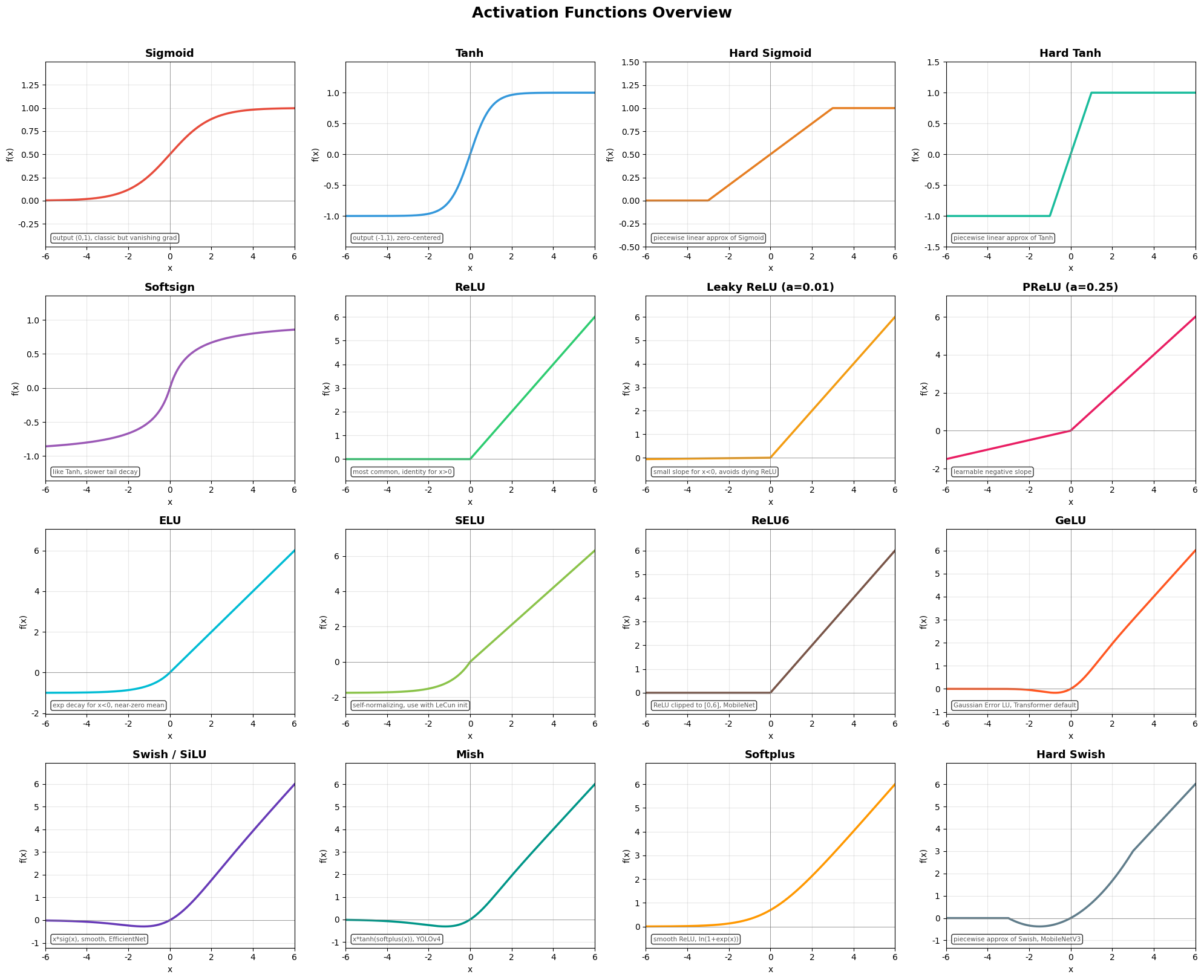
all_funcs = [
('Sigmoid', sigmoid(x), '#e74c3c', 'output (0,1), classic but vanishing grad'),
('Tanh', tanh_fn(x), '#3498db', 'output (-1,1), zero-centered'),
('Hard Sigmoid', hardsigmoid(x), '#e67e22', 'piecewise linear approx of Sigmoid'),
('Hard Tanh', hardtanh(x), '#1abc9c', 'piecewise linear approx of Tanh'),
('Softsign', softsign(x), '#9b59b6', 'like Tanh, slower tail decay'),
('ReLU', relu(x), '#2ecc71', 'most common, identity for x>0'),
('Leaky ReLU (a=0.01)', leaky_relu(x), '#f39c12', 'small slope for x<0, avoids dying ReLU'),
('PReLU (a=0.25)', prelu(x), '#e91e63', 'learnable negative slope'),
('ELU', elu(x), '#00bcd4', 'exp decay for x<0, near-zero mean'),
('SELU', selu(x), '#8bc34a', 'self-normalizing, use with LeCun init'),
('ReLU6', relu6(x), '#795548', 'ReLU clipped to [0,6], MobileNet'),
('GeLU', gelu(x), '#ff5722', 'Gaussian Error LU, Transformer default'),
('Swish / SiLU', swish(x), '#673ab7', 'x*sig(x), smooth, EfficientNet'),
('Mish', mish(x), '#009688', 'x*tanh(softplus(x)), YOLOv4'),
('Softplus', softplus(x), '#ff9800', 'smooth ReLU, ln(1+exp(x))'),
('Hard Swish', hardswish(x), '#607d8b', 'piecewise approx of Swish, MobileNetV3'),
]
n = len(all_funcs)
cols = 4
rows = (n + cols - 1) // cols
fig, axes = plt.subplots(rows, cols, figsize=(5 * cols, 4 * rows))
axes = axes.flatten()
for i, (name, y, color, desc) in enumerate(all_funcs):
ax = axes[i]
ax.plot(x, y, color=color, linewidth=2.5)
ax.axhline(y=0, color='gray', linewidth=0.5)
ax.axvline(x=0, color='gray', linewidth=0.5)
ax.set_title(name, fontsize=13, fontweight='bold')
ax.set_xlabel('x', fontsize=10)
ax.set_ylabel('f(x)', fontsize=10)
ax.set_xlim(-6, 6)
y_min, y_max = y.min(), y.max()
margin = max((y_max - y_min) * 0.15, 0.5)
ax.set_ylim(y_min - margin, y_max + margin)
ax.grid(True, alpha=0.3)
ax.text(0.03, 0.03, desc, transform=ax.transAxes, fontsize=7.5,
color='#555', verticalalignment='bottom',
bbox=dict(boxstyle='round,pad=0.3', facecolor='white', alpha=0.8))
for j in range(n, len(axes)):
axes[j].set_visible(False)
plt.suptitle('Activation Functions Overview', fontsize=18, fontweight='bold', y=1.01)
plt.tight_layout()
plt.savefig('activation_functions_individual.png', dpi=150, bbox_inches='tight')
plt.show()
print(f'{n} activation functions plotted.')
# ============================================================
# Grouped comparison (3 subplots)
# ============================================================
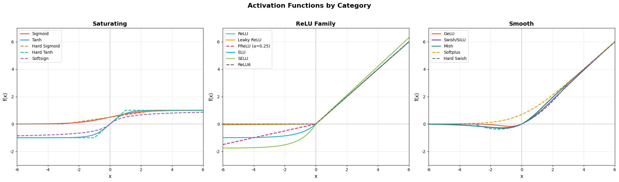
groups = {
'Saturating': [
('Sigmoid', sigmoid(x), '#e74c3c', '-'),
('Tanh', tanh_fn(x), '#3498db', '-'),
('Hard Sigmoid', hardsigmoid(x), '#e67e22', '--'),
('Hard Tanh', hardtanh(x), '#1abc9c', '--'),
('Softsign', softsign(x), '#9b59b6', '--'),
],
'ReLU Family': [
('ReLU', relu(x), '#2ecc71', '-'),
('Leaky ReLU', leaky_relu(x), '#f39c12', '-'),
('PReLU (a=0.25)', prelu(x), '#e91e63', '--'),
('ELU', elu(x), '#00bcd4', '-'),
('SELU', selu(x), '#8bc34a', '-'),
('ReLU6', relu6(x), '#795548', '--'),
],
'Smooth': [
('GeLU', gelu(x), '#ff5722', '-'),
('Swish/SiLU', swish(x), '#673ab7', '-'),
('Mish', mish(x), '#009688', '-'),
('Softplus', softplus(x), '#ff9800', '--'),
('Hard Swish', hardswish(x), '#607d8b', '--'),
],
}
fig, axes = plt.subplots(1, 3, figsize=(21, 6))
for ax, (group_name, funcs) in zip(axes, groups.items()):
for name, y, color, ls in funcs:
ax.plot(x, y, label=name, color=color, linestyle=ls, linewidth=2)
ax.axhline(y=0, color='gray', linewidth=0.5)
ax.axvline(x=0, color='gray', linewidth=0.5)
ax.set_title(group_name, fontsize=14, fontweight='bold')
ax.set_xlabel('x', fontsize=12)
ax.set_ylabel('f(x)', fontsize=12)
ax.legend(fontsize=10, loc='upper left')
ax.set_xlim(-6, 6)
ax.set_ylim(-3, 7)
ax.grid(True, alpha=0.3)
plt.suptitle('Activation Functions by Category', fontsize=16, fontweight='bold', y=1.02)
plt.tight_layout()
plt.savefig('activation_functions_grouped.png', dpi=150, bbox_inches='tight')
plt.show()
# ============================================================
# All-in-one overlay
# ============================================================
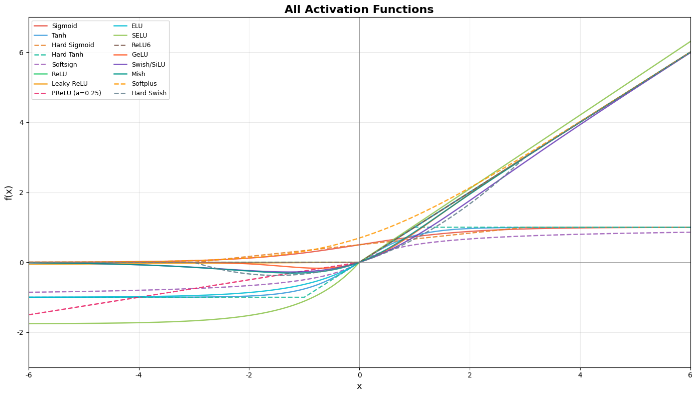
all_flat = [item for g in groups.values() for item in g]
fig, ax = plt.subplots(figsize=(14, 8))
for name, y, color, ls in all_flat:
ax.plot(x, y, label=name, color=color, linestyle=ls, linewidth=1.8, alpha=0.85)
ax.axhline(y=0, color='gray', linewidth=0.5)
ax.axvline(x=0, color='gray', linewidth=0.5)
ax.set_title('All Activation Functions', fontsize=16, fontweight='bold')
ax.set_xlabel('x', fontsize=13)
ax.set_ylabel('f(x)', fontsize=13)
ax.legend(fontsize=9, loc='upper left', ncol=2)
ax.set_xlim(-6, 6)
ax.set_ylim(-3, 7)
ax.grid(True, alpha=0.3)
plt.tight_layout()
plt.savefig('activation_functions_all.png', dpi=150, bbox_inches='tight')
plt.show()2、激活函数可视化
3、激活函数总览表
| 序号 | 函数名称 | 数学公式 | 输出范围 | 特点 | 优点 | 缺点 | 推荐使用场景 |
|---|---|---|---|---|---|---|---|
| 1 | Sigmoid | (0, 1) | S型曲线,中心不对称 | 输出可解释为概率,平滑可导 | 梯度饱和(两端近零),非零中心,指数计算开销大 | 二分类输出层(需配合交叉熵);早期RNN门控(已被tanh替代) | |
| 2 | Tanh | (-1, 1) | 零中心,S型曲线 | 零中心有助于梯度更新,梯度比Sigmoid陡峭 | 仍有饱和区域(梯度消失),计算稍复杂 | RNN隐藏层;生成模型中间层;特征映射需负值时 | |
| 3 | Hard Sigmoid | (0, 1) | 分段线性近似 | 计算极快,无指数运算 | 导数分段常数(非光滑),近似精度较低 | 移动端/嵌入式部署(如MobileNet);需快速推理且精度要求不高时 | |
| 4 | Hard Tanh | [-1, 1] | 分段线性截断 | 极简计算,无饱和区(截断区梯度=0) | 截断处梯度突变,训练时可能梯度消失 | 约束特征范围;某些强化学习策略网络;轻量级模型 | |
| 5 | Softsign | (-1, 1) | 类似Tanh,但多项式衰减 | 比Tanh更平滑的尾部,渐近线更缓 | 仍存在饱和,计算除法稍慢 | 需要比Tanh更稳定梯度的极深网络(较少使用) | |
| 6 | ReLU | [0, ∞) | 单边抑制,线性正部 | 计算极快,稀疏激活,缓解梯度消失 | 神经元“死亡”(负区间梯度0),输出非零中心 | 深度CNN隐藏层默认首选;全连接层 | |
| 7 | Leaky ReLU | (通常α=0.01) | (-∞, ∞) | 负区间保留小斜率 | 避免神经元死亡,梯度始终非零 | α需手动设定,对负值响应弱 | 避免ReLU死亡问题的CNN;RNN;生成对抗网络 |
| 8 | PReLU | (-∞, ∞) | 负斜率可学习 | 自适应负斜率,理论上优于固定α | 增加参数量(每通道或每层一个α),易过拟合 | 大型CNN且数据充足时(如ImageNet分类) | |
| 9 | ELU | (常用α=1) | (-α, ∞) | 负区间指数趋近-α | 输出均值近零,负区间饱和抗噪声 | 计算含指数,稍慢;α需调参 | 噪声较强的任务;需要自归一化特性的网络 |
| 10 | SELU | λ≈1.0507,α≈1.6733 | (-λα, ∞) | 自归一化激活 | 可使网络输出自动归一化(均值0方差1) | 必须配合LeCun初始化;对输入尺度敏感 | 全连接“自归一化神经网络”(SNN);MLP深层结构 |
| 11 | ReLU6 | [0, 6] | 截断ReLU | 限制输出范围利于低精度推理(如FP16) | 饱和区梯度0,可能信息损失 | 移动端量化模型(MobileNet系列);有界特征输出 | |
| 12 | GeLU | ≈0.5x[1+tanh(√(2/π)(x+0.044715x³))] | (-∞, ∞) | 随机正则激活 | Transformer首选,结合Dropout思想 | 计算复杂(含tanh和三次方) | Transformer(BERT,GPT);自然语言处理 |
| 13 | Swish / SiLU | (β=1时称SiLU) | (-∞, ∞) | 自门控激活 | 光滑,下界无饱和,上界无界,性能优于ReLU | 计算量稍大(含sigmoid) | 深层CNN(EfficientNet);需平滑梯度的任务 |
| 14 | Mish | (-∞, ∞) | 自门控变体 | 光滑且几乎处处非单调,性能常优于Swish | 计算最复杂(含tanh和exp/log) | 目标检测(YOLOv4,YOLOv5);图像分割 | |
| 15 | Softplus | (0, ∞) | 平滑ReLU | 处处光滑,无硬拐点 | 计算含log/exp,梯度饱和区(x«0) | 需要可微且正数输出的场合(如方差预测);概率模型 | |
| 16 | Hard Swish | [0, ∞) | 分段线性近似Swish | 计算极快,适合移动端 | 非光滑,近似误差 | 移动端CNN(MobileNetV3);低功耗推理 |
4、详细分类与选择指南
2.1 饱和型激活函数
- Sigmoid / Tanh / Softsign:适用于需要概率输出或对称输出的浅层网络,但梯度消失严重,不建议在深层网络隐藏层使用。
- Hard Sigmoid / Hard Tanh:作为替代方案,用于移动端或需要快速推理的模型。
2.2 ReLU 及其变体
- ReLU:深度CNN默认首选,简单高效。
- Leaky ReLU / PReLU:当观察到大量神经元死亡时,改用Leaky ReLU;有充足数据时可尝试PReLU。
- ELU / SELU:需要自归一化或抗噪声时选用SELU(需配合特定初始化);ELU适合中等深度网络。
- ReLU6:量化模型或移动端部署时推荐。
2.3 现代平滑/自门控激活函数
- GeLU:Transformer模型的标配,NLP任务优先选择。
- Swish / SiLU:大型CNN(如EfficientNet)中常优于ReLU,且SiLU是PyTorch原生实现。
- Mish:追求极致精度时可尝试,尤其在目标检测中表现突出,但计算代价高。
- Hard Swish:移动端替代Swish的实用选择。
- Softplus:需要光滑正输出的回归任务(如预测方差)。
5、实用选择决策树
开始
│
├─ 任务是否为二分类输出层? ── 是 ──→ Sigmoid
│
├─ 是否为RNN或生成模型隐藏层? ── 是 ──→ Tanh
│
├─ 是否为Transformer/NLP模型? ── 是 ──→ GeLU
│
├─ 是否部署到移动端/边缘设备? ── 是 ──→ Hard Swish / ReLU6 / Hard Tanh
│
├─ 是否遇到神经元死亡问题? ── 是 ──→ Leaky ReLU 或 ELU
│
├─ 是否希望自归一化(MLP深层)? ── 是 ──→ SELU(+LeCun初始化)
│
├─ 是否追求最高精度且算力充足? ── 是 ──→ Mish / Swish
│
└─ 默认选择 ──→ ReLU(CNN) 或 GeLU(Transformer)
4. 注意事项
- 梯度消失:避免在深层网络中使用Sigmoid/Tanh作为隐藏层激活。
- 计算效率:Hard形式的函数(Hard Swish等)在CPU/移动端比指数版本快数倍。
- 初始化匹配:SELU需要配合LeCun正态初始化;ReLU族通常配合He初始化;Tanh配合Xavier初始化。
- 可学习参数:PReLU增加参数量,需注意正则化。
- 输出范围:有界输出(如Sigmoid/Tanh)适合作为最终层,但会限制特征表达能力。